ufjc.examples.approaches module
An example module comparing isotensional approaches.
This module contains a main function that allows the comparison of
different approaches of obtaining the single-chain mechanical response of
a given single-chain model in the isotensional ensemble.
The results are plotted using matplotlib.
When executed at the command line, flags are passed as keyword arguments.
Example
Compare approaches, using 1000 samples for the Monte Carlo approach:
python -m ufjc.examples.approaches --num_samples 1000
- main(**kwargs)[source]
Main function for the module.
This is the main function, called when executing the module from the command line, also available when importing the module.
- Parameters:
**kwargs – Arbitrary keyword arguments. Passed to
uFJCinstantiation.
Example
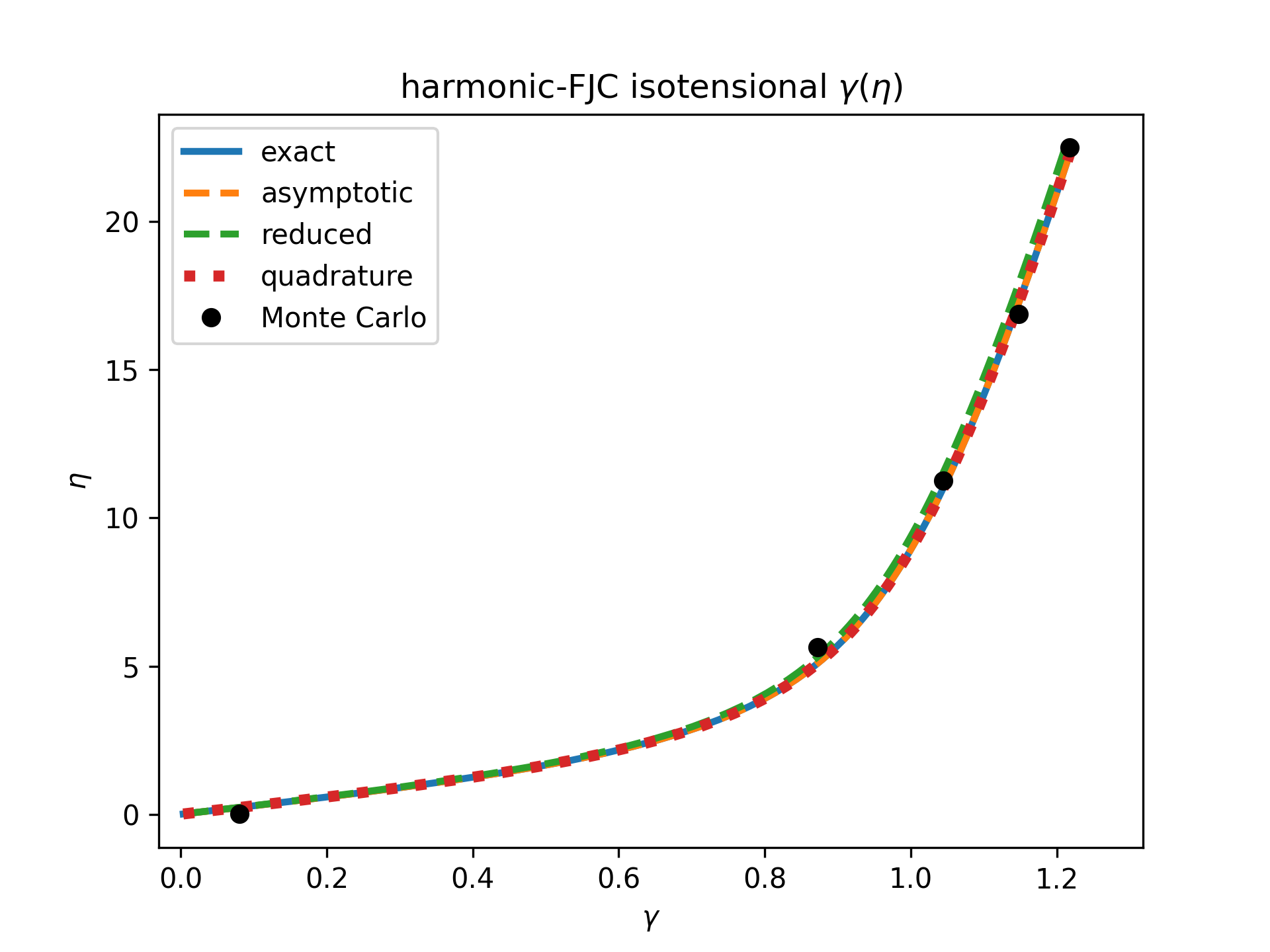
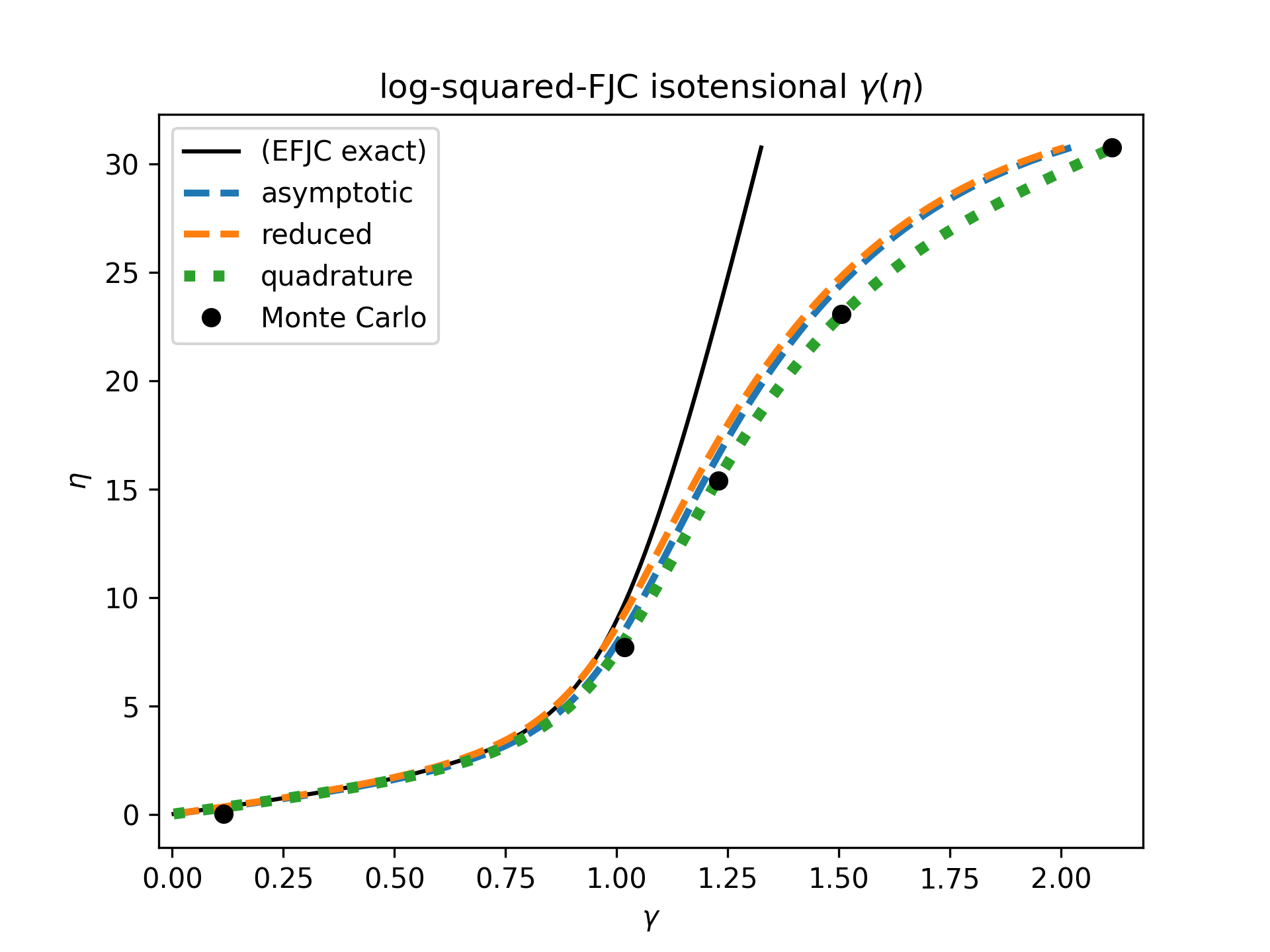
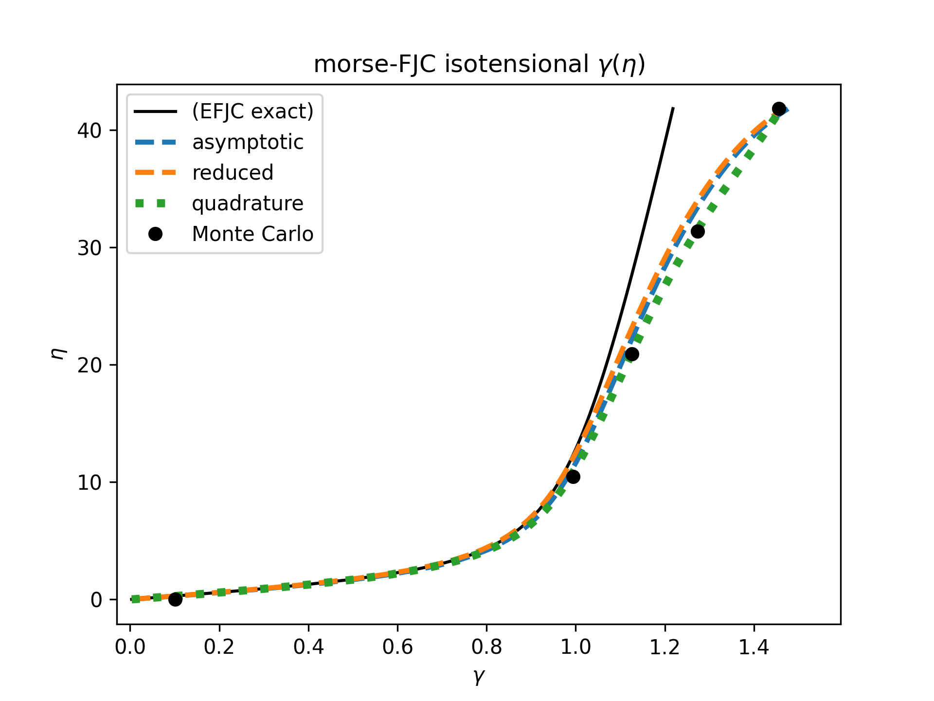
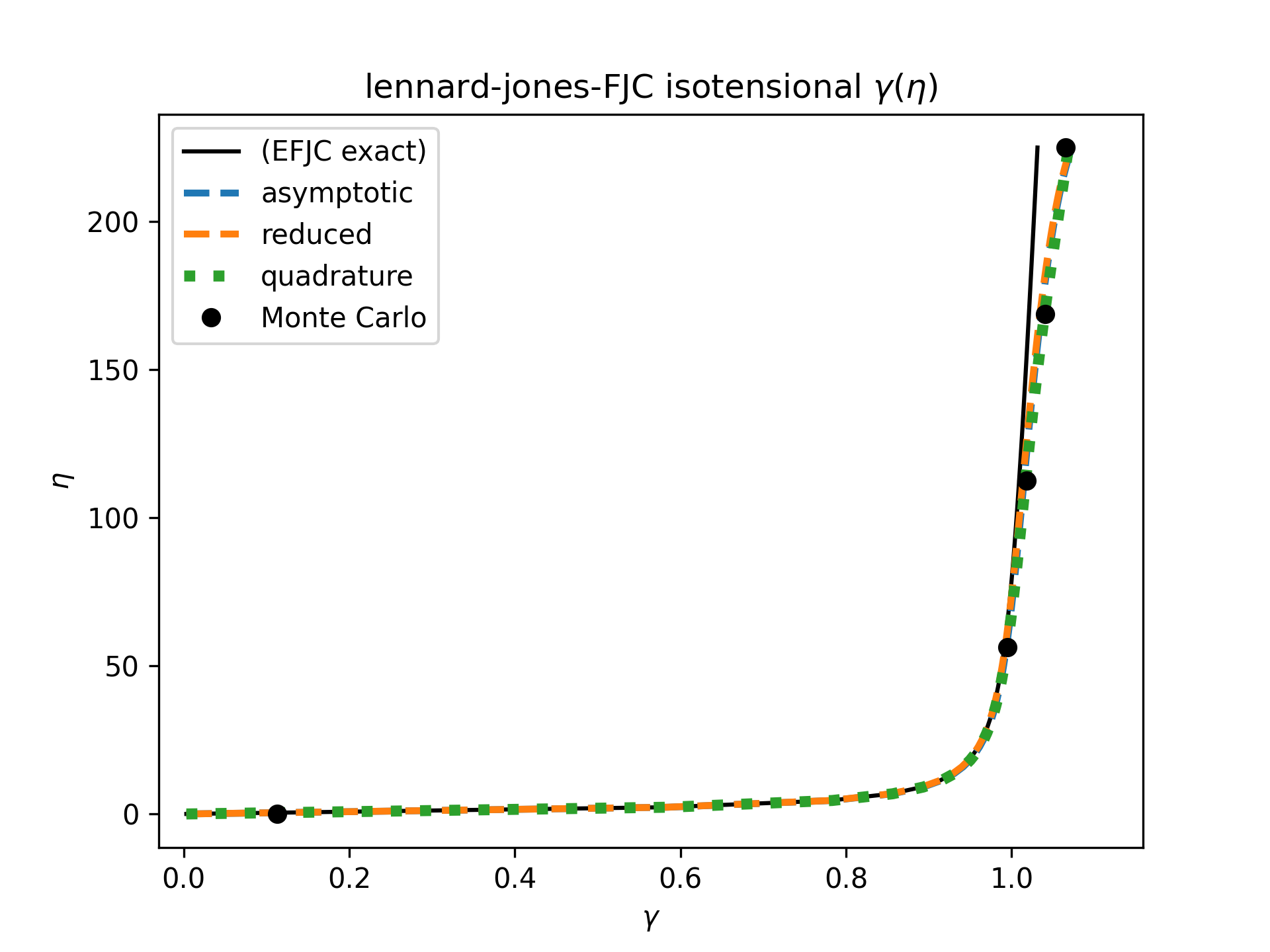
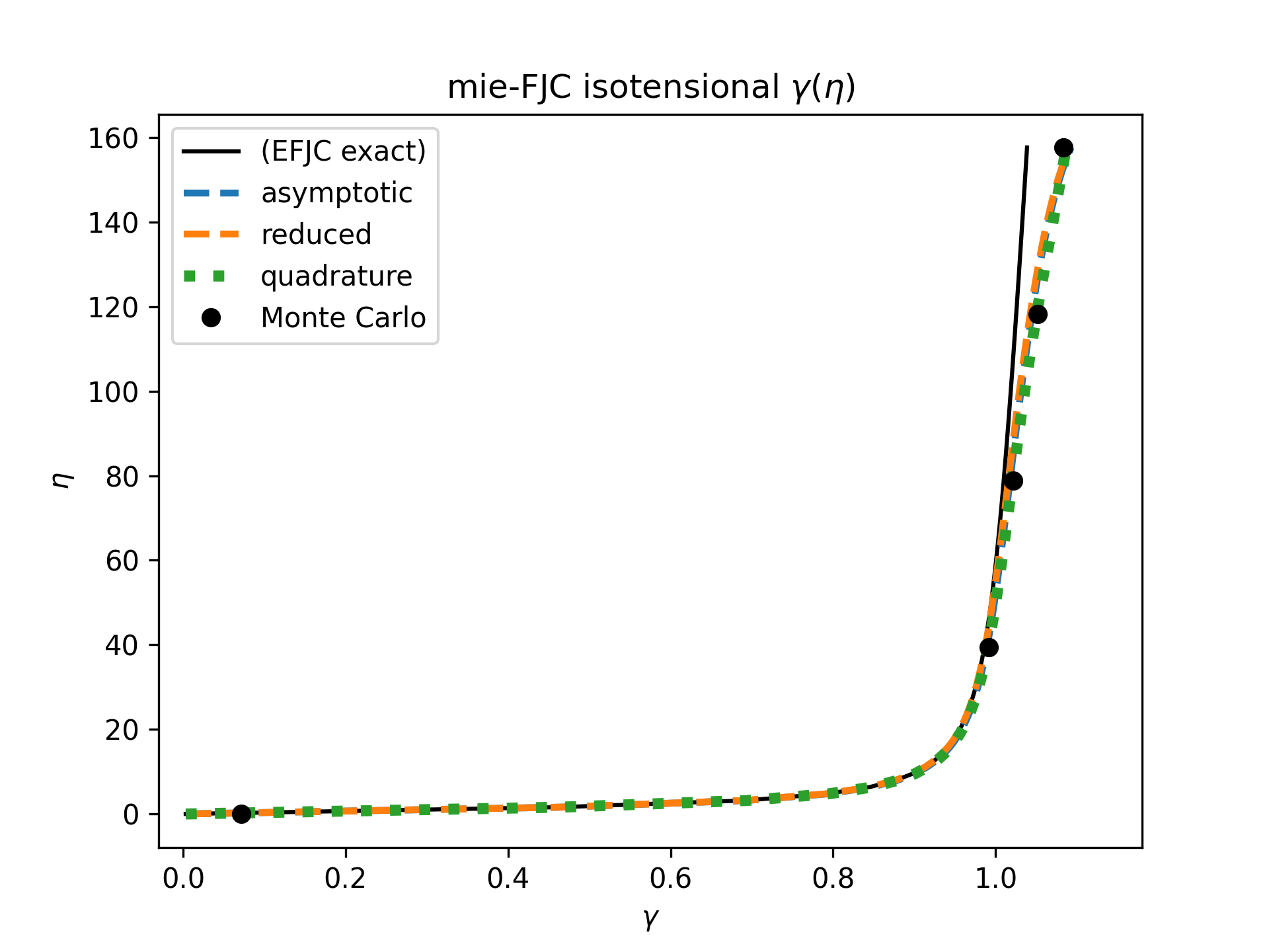
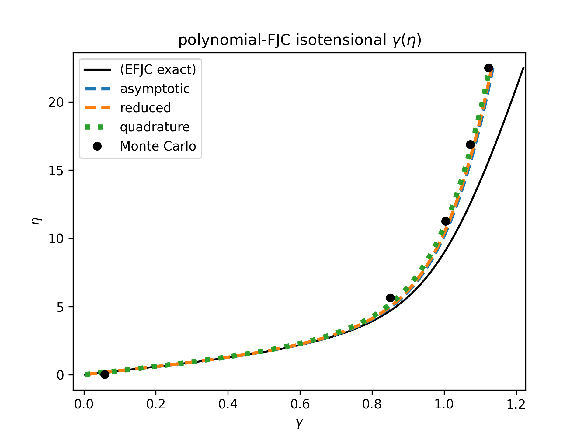
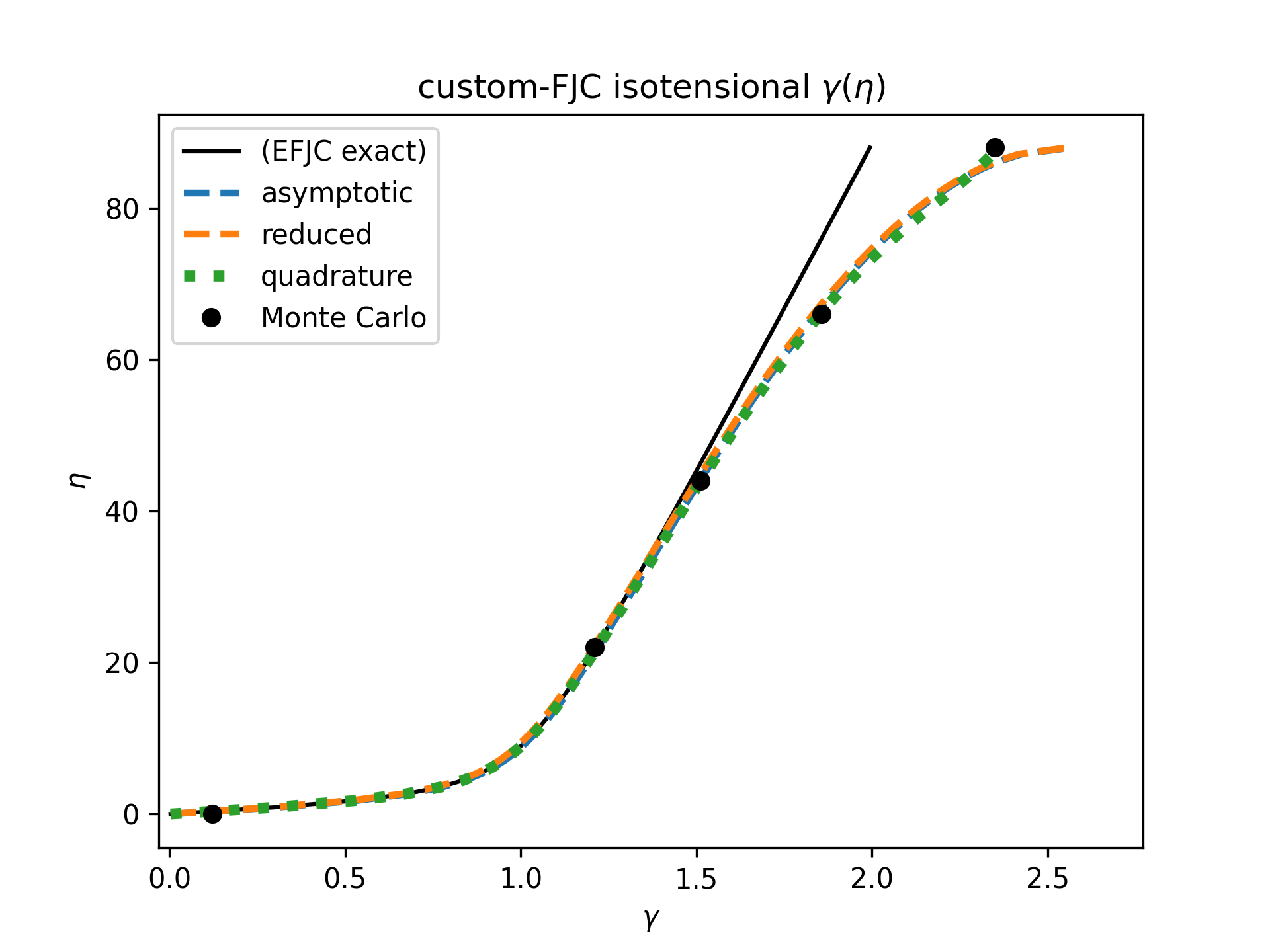
Plot and compare each approach for each available potential, including examples of polynomial and fully custom potentials, for \(\varepsilon=88\), keeping the harmonic result (EFJC) as a comparison for non-harmonic cases:
>>> import numpy as np
>>> from ufjc.examples import approaches
>>> approaches.main(potential='harmonic')
>>> approaches.main(potential='log-squared')
>>> approaches.main(potential='morse')
>>> approaches.main(potential='lennard-jones')
>>> approaches.main(potential='mie', n=10, m=4)
>>> approaches.main(potential='polynomial',
...     coefficients=[1, 2, 3])
>>> approaches.main(potential='custom',
...     varepsilon=88,
...     phi=lambda lambda_: 1 - np.cos(lambda_ - 1),
...     eta_link=lambda lambda_: 88*np.sin(lambda_ - 1),
...     delta_lambda=lambda eta: np.arcsin(eta/88),
...     kappa=88,
...     c=2/3,
...     lambda_max=1 + np.pi/2,
...     eta_max=88)